invasion (3 to 10 g, Stenman
et al.
1999), indicating
that most cancers could be detected while they were
organ limited. But would they be detected? That
depends upon the screening program schedule. If,
for example, the schedule called for a single PSA
determination at the age of 50 years, prostate
cancers would be detected only in those men who
had a cancer that had already reached a detectable
size. They would represent only a fraction of the
individuals who would eventually have symptomatic
prostate cancer. If, on the other hand, the PSA
concentration were measured yearly after the age of
50 years, almost every cancer would be detected
before capsular invasion. This is so because it takes
about 13 years for a prostate cancer to grow from
0.22 g to 3 grams (see Figure 11.2; 0.22 g and 3 g
equate to diameters of 7.5 and 18 mm, respectively).
Thus, many screening studies would be performed
on every man harboring a prostate cancer while the
cancer was detectable and pre-invasive. An optimal
screening schedule is one in which the screening
study is performed once during the screening
window. If a sensitivity of 0.95 were to be consid-
ered the minimal acceptable screening performance,
the screening window for PSA would be 13 years,
from a tumor mass of 0.22 g to a mass of 3 g.
Performing the screening study on a schedule of
once every 13 years would therefore be optimal. To
account for possible lapses in the regularity of
obtaining a screening study, a PSA determination
every 10 years might be recommended. A problem
with this analysis is, of course, that it applies to only
a few men, those with normal prostate glands. By
the time they reach their fifties, an age at which
starting to screen for prostate cancer is reasonable
based on the natural history of the disease, most men
have developed some degree of BPH. This means
that there is an appreciable background plasma PSA
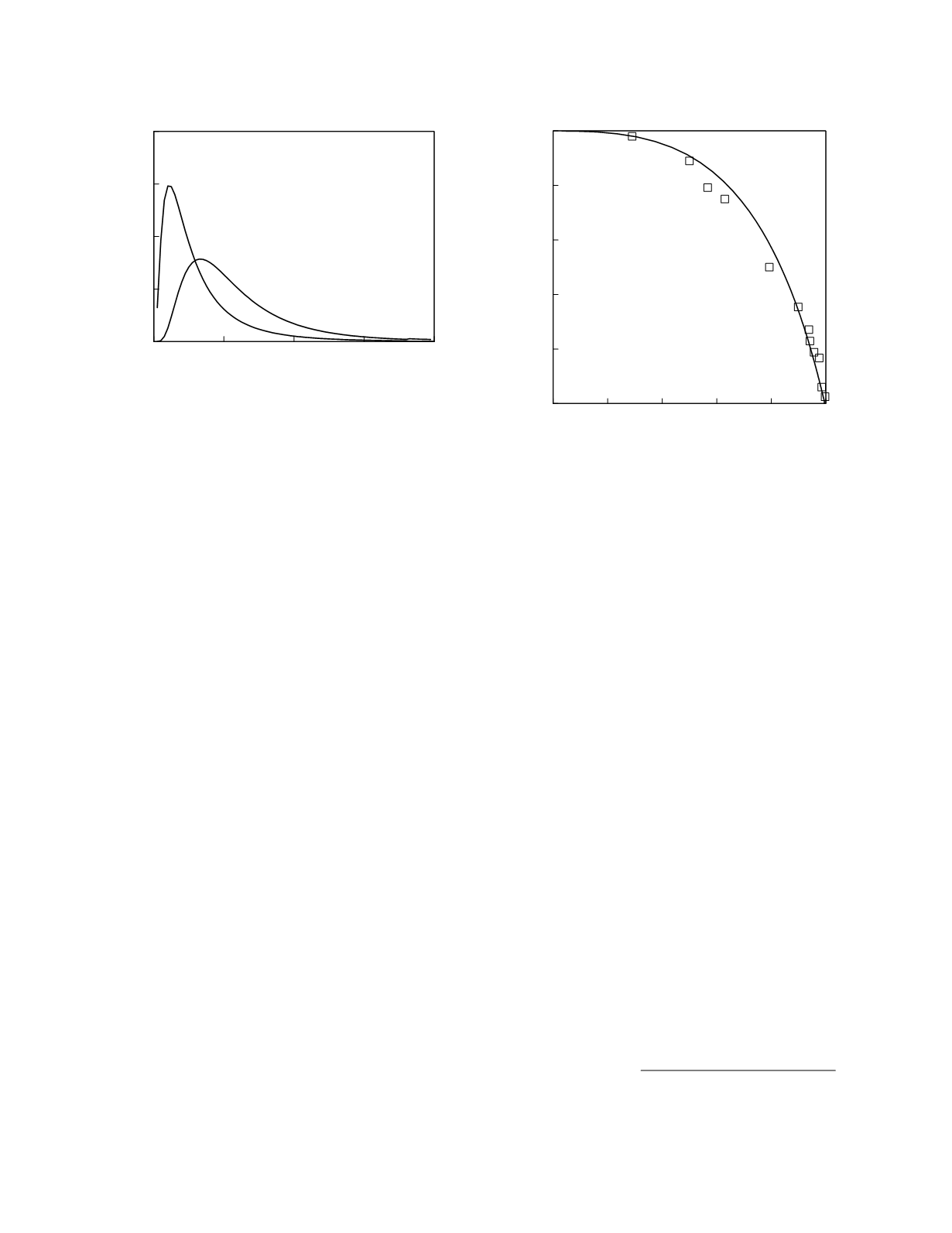
concentration. Figure 11.3 shows population
frequency distributions for plasma PSA concentra-
tion. The PSA concentrations in men without cancer
are due entirely to the presence of BPH; the PSA
concentrations in men with cancer are due to cancer
and concomitant BPH (Partin
et al.
1990). There is
a considerable overlap in the frequency distributions
of the two populations. Consequently, screening for
prostate cancer in the male population as a whole
necessitates a tradeoff between screening sensitivity
and specificity. For unscheduled, or one-time,
screening among men 50 to 59 years old, the trade-
off is as shown in Figure 11.4 (for a similar analysis
of a different data set read the article by Meigs
et al.
1996). To determine the critical screening value for
the plasma PSA concentration in this setting, the
threshold likelihood ratio for followup must be
calculated. This is done using the formula,
threshold likelihood ratio for followup =
(
1
−
prevalence
)
P
[
rejection
]
prevalence
(
1
−
P
[
rejection
])
where P[rejection] is the threshold posterior
probability for rejection of the diagnosis of prostate
Cancer
11-8
Figure 11.3
Reference frequency distributions for plasma
PSA concentration. The curves represent lognormal
frequency distributions fit to the data reported by Catalona
et al.
(1994) for men 50 to 59 years old.
0
5
10
15
20
Plasma PSA concentration (µg/L)
0
0.1
0.2
0.3
0.4
Frequency
Cancer free
Cancer
0
0.2
0.4
0.6
0.8
1
Specificity
0
0.2
0.4
0.6
0.8
1
Sensitivity
Figure 11.4
ROC curves for screening for prostate cancer
using plasma PSA concentration. The squares represent
the data reported by Catalona
et al.
(1994) for men 50 to 59
years old. The continuous line is the curve constructed from
lognormal frequency distributions of the data.


