Janovski complex. The signal consists of the reduc-
tion in the amount of light passing through the
reaction solution. The signal is detected by a
spectrophotometer.
Calculation of results
In order to arrive at a study result, the magni-
tude of the signal generated by a sample must be
converted to a concentration value. This can be
done in either of two ways. If the measurement
system has been shown to have signal generating
properties that closely match the theoretical ideal,
the theoretical relationship between analyte concen-
tration and signal magnitude can be used to calculate
the result. For example, the theoretical relationship
between analyte concentration and light absorbance
is embodied in the Beer-Lambert law,
analyte concentration =
absorbance
analyte absorptivity
$
light path
For an ideal system, dividing the observed absor-
bance value by the known values for the absorptivity
of the analyte and the length of the light path in the
detector yields the analyte concentration.
In practice, the behavior of measurement
systems is rarely ideal, so the use of theoretical
relationships is not a satisfactory way to calculate
results. Instead, results are calculated using the
empirical relationship between analyte concentration
and signal magnitude as established by the measure-
ment of signals produced by a set of test materials
with known analyte concentrations. These test
materials are called calibrators (formerly, standards)
and the relationship between analyte concentration
and signal magnitude is called a calibration curve.
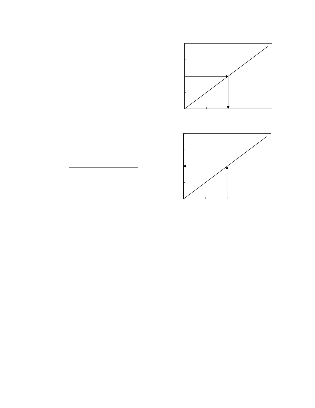
A hypothetical linear calibration curve is shown in
the upper graph of Figure 2.1
To convert the signal generated by a test sample
to a concentration value, the calibration curve is
used in reverse. That is, rather than finding the y
(signal) value on the curve for a known x (concen-
tration) value, an x value on the curve is found that
corresponds to the known y value. For a signal of
100 units, for instance, the corresponding point on
the calibration curve has a concentration of 10 units.
The measurement result is therefore, 10 concentra-
tion units. Because it is unconventional to reverse
the roles of the x- and y-axes, results are calculated
using what is called a measurement curve which is
identical to the calibration curve except that the x-
and y-axes are switched (the lower graph in Figure
2.1). Note that inversion of the equation describing
the calibration curve yields the equation that defines
the measurement curve.
Calibration and measurement curves are usually
constructed each time that a batch of measurements
is made. Calibrators are run along with the test
samples and the parameters of the equations defining
the curves are estimated from the observed calibrator
and signal magnitude pairs. The number and
spacing of the calibrators should be chosen with the
intent of providing for highly reliable estimation of
the equation parameters. According to the statistical
theory of optimal design, there exists a unique set of
calibrator concentrations that yields the most precise
estimates of the equation parameters (Fedorov 1972,
Steinberg and Hunter 1984). In general, the number
of separate concentrations that should be evaluated
equals the number of parameters in the equation. In
the case of a linear calibration curve there are two
Laboratory Methods
2-2
0
5
10
15
20
Calibrator concentration
0
50
100
150
200
Signal magnitude
0
50
100
150
200
Signal magnitude
0
5
10
15
20
Sample concentration
calibration
y = b0 + b1 x
measurement
y = (x - b0) / b1
Figure 2.1
Hypothetical calibration and measurement
curves (solid lines). The graphical technique for the calcula-
tion of the result given a signal of 100 units is depicted.


