result in only 0.1 percent rather than 2.3 percent of
the control sample results having values smaller than
the established mean minus 2 SD
within-laboratory
. The net
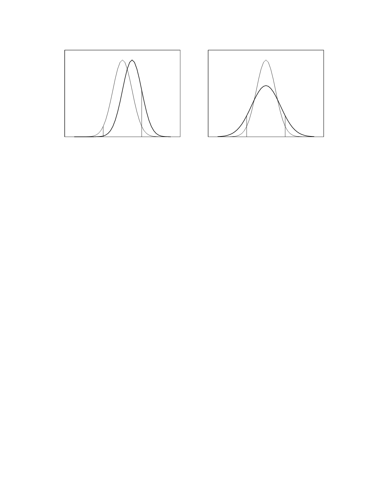
effect of the bias is an overall increase in the
percentage of control sample results outside of the
central region of the established distribution, 16.0
percent versus 4.6 percent. Identical percentages
apply when the bias is negative.
If there is an increase in method imprecision,
there will be an increased probability for the control
sample results to be in the region of the tails of the
established distribution. An example of this is
shown in the graph on the right in Figure 2.4. For a
1.5-fold increase in imprecision, 9.1 percent of the
control sample results will be more than 2
SD
within-laboratory
larger than the established mean and
9.1 percent of the control sample results will be
more than 2 SD
within-laboratory
smaller than the estab-
lished mean. Hence, the net effect of the increase in
imprecision is an overall increase from 4.6 to 18.2
in the percentage of control sample results outside of
the central region of the established distribution.
In general, there is an increased probability for
control sample results to be more than 2
SD
within-laboratory
larger or smaller than the established
mean if there is currently a bias in the method or an
increase in the imprecision of the method. There-
fore, a control sample result of this magnitude can
be taken as a indication of a reduction in method
quality. This is the statistical basis of the 1
2s
control
rule: a batch of measurements should not be consid-
ered to be in-control if one control result exceeds the
mean plus or minus 2 SD
within-laboratory
.
The performance of this control rule, or any control
rule, is characterized by the relationship between the
probability of rejecting a batch using the rule and the
magnitude of the current change in quality in the
method. This graphical presentation of this relation-
ship is called the operating characteristic curve.
Figure 2.5 shows the operating characteristic curves
for the 1
2s
control rule when using one to five
control samples per batch. These curves represent
the operating characteristics of the 1
2s
control rule
for detecting current bias; operating characteristic
curves can also be drawn for the detection of
increased imprecision and a 3-dimensional surface
can be used to present the operating characteristics
for the simultaneous detection of bias and increased
imprecision. A bias of zero means that the quality
of the method is unchanged so a rejection of a batch
at this value represents a false rejection. Thus, the
y-intercepts of the curves equal the rates of false
rejection when using the indicated number of control
samples.
In the quality control of a particular method, the
control rule that should be used is the one that most
closely achieves the clinical quality control goals for
performance and false-rejection rate while minimiz-
ing the number of control samples run per batch.
Consider, for instance, a method for which the false-
rejection rate goal is 5 percent and the performance
goal is 90 percent rejection of batches for which the
current method bias is equal to or greater than 2.5
SD
within-laboratory
. Using the 1
2s
control rule, two
control samples must be run per batch to achieve the
performance goal at the stipulated level of bias.
Laboratory Methods
2-10
40
60
80 100 120 140 160
Control sample concentration (µmol/L)
Frequency
40
60
80 100 120 140 160
Control sample concentration (µmol/L)
Frequency
established
current
current
- 2 SD
+ 2 SD
- 2 SD
+ 2 SD
established
Figure 2.4
Frequency distributions of control sample results for a hypothetical laboratory method. The established distribu-
tion has a mean of 100 µmol/L and an SD
within-laboratory
of 10 µmol/L. It is shown as a light curve in both graphs. The current
distributions are shown as dark curves. In the graph on the left, the method currently has a bias of 10 µmol/L. In the graph
on the right, the SD
within-laboratory
of the method is currently 15 µmol/L.


