However, with two control samples per batch, the
false-rejection rate is too high, 8.9 percent. Using
the 1
3s
control rule (which states that a batch of
measurements should not be considered to be
in-control if one control result exceeds the mean plus
or minus 3 SD
within-laboratory
), an acceptable false-
rejection rate, 1.6 percent, can be achieved at the
performance goal, but at the expense of requiring six
control samples per batch. Fewer control samples
per batch can be used while still achieving the
quality control goals if a control rule intermediate
between the 1
2s
and 1
3s
rules is employed. Specifi-
cally, using three control samples per batch, the
1
2.385s
rule will yield a 5 percent false-rejection rate
and a 90.6 percent rejection rate. In general, the
best control rules in terms of control sample require-
ments are those for which the control limits have
been calculated to achieve the specific quality
control goals (Bishop and Nix 1993).
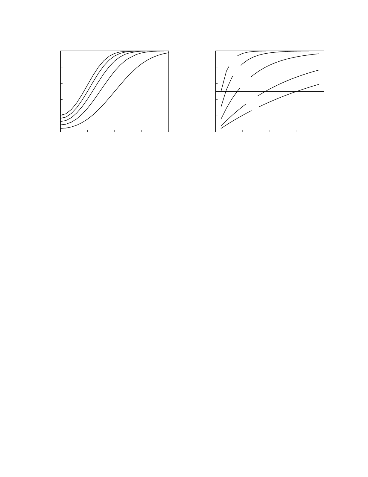
A somewhat different approach to evaluating
control performance is taken when considering the
detection of long-term, or persistent, quality degra-
dation in a method. Here the focus is on how many
batches will be accepted before the control rule leads
to a batch rejection and, thereby, detection of the
quality problem (Nix
et al.
1987). The most infor-
mative way to present this performance behavior is
as the cumulative run length distribution for the
control rule. This distribution gives the probability
of having rejected any batch, including the current
batch, as a function of the number of batches run
since the inception of the quality problem. Figure
2.6 shows the cumulative run length distributions for
the 1
2s
rule at five different levels of persistent
method bias. The graph also has a line that indicates
the medians of the distributions. For instance, the
median run length for zero method bias is 15
batches. That is the median number of consecutive
batches that can be expected to be accepted using
this control rule when the quality of the method is
unchanged. The median run lengths for the other
levels of persistent method bias in the graph are 9,
4, 2, and 1, in order of increasing bias. (Note:
average run length is the usual measure for the
evaluation of control rules in the setting of a persis-
tent problem in method quality. Because run length
frequency distributions are highly right-skewed,
average run lengths will be larger than median run
lengths. For example, the average run length for the
1
2s
control rule is 22 batches when the quality of the
method is unchanged. Compare this to the median
value of 15 batches. Because it is less influenced by
extreme run length values of low probability, median
run length better reflects the run length behavior
expected of a control rule.)
The control rule used to monitor a method for
persistent quality degradation must satisfy the clini-
cal performance and false-rejection quality control
goals for such problems. The performance goal can
be expressed as maximum median (or average) run
length at a specified level of quality decline in the
method. The false-rejection quality goal can be
expressed either as an acceptable median run length
when the quality of the method is unchanged or, as
for single-batch quality monitoring, as an acceptable
false-rejection rate per batch. Typically, single rule
control procedures are not able to provide the
Laboratory Methods
2-11
Figure 2.5
Operating characteristic curves for the detection
of current method bias using the 1
2s
control rule. Curves
are shown for one to five control samples per batch.
0
1
2
3
4
Bias (multiples of within-laboratory SD)
0
0.2
0.4
0.6
0.8
1
Rejection probability
n =1
n = 5
0
5
10
15
20
Run length
0
0.2
0.4
0.6
0.8
1
Rejection probability
0
0.5
1.0
1.5
2.0
Figure 2.6
Cumulative run length distributions for the
detection of persistent method bias using the 1
2s
control
rule. Curves are shown for method bias in half multiples of
SD
within-laboratory
.


