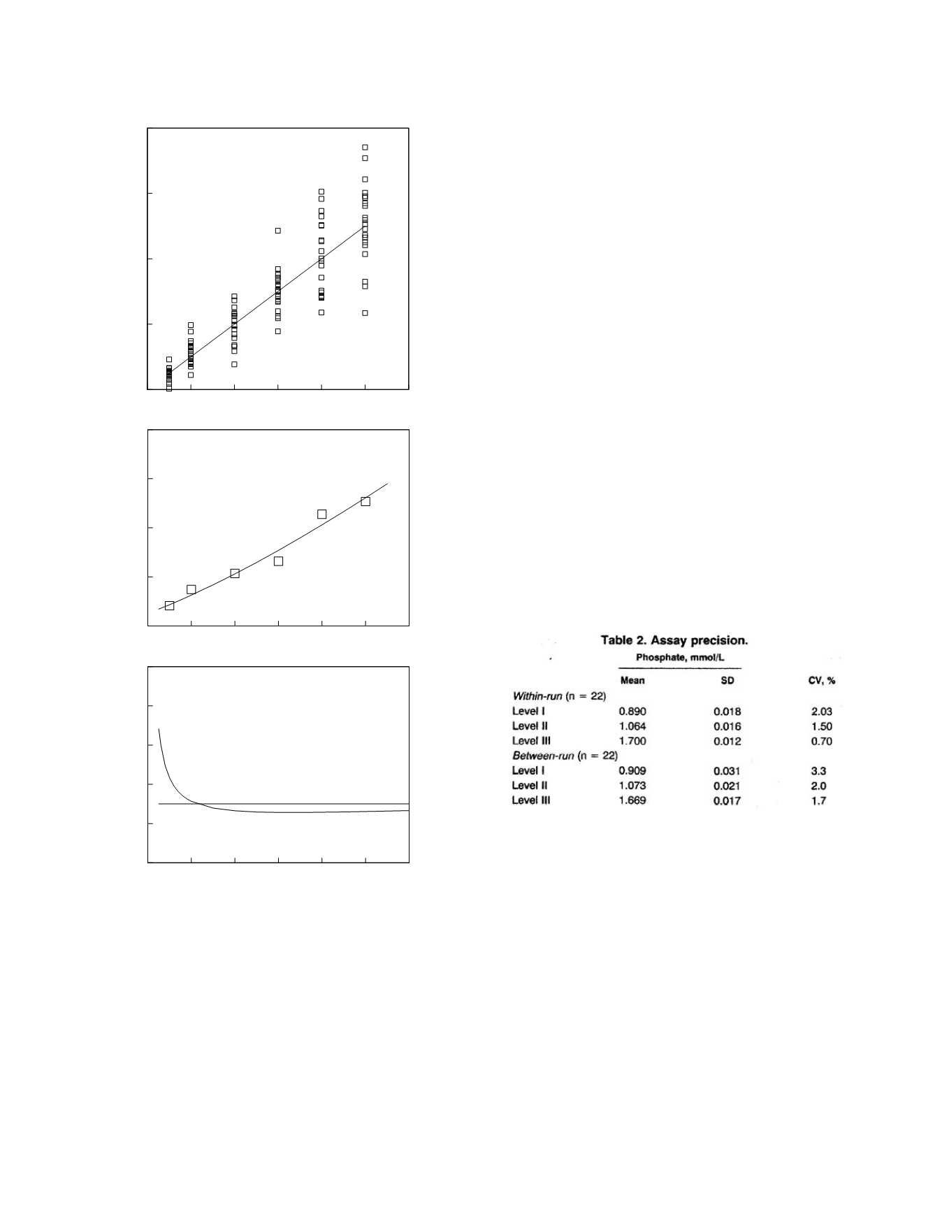
The graph of the imprecision model was origi-
nally called a precision profile (Ekins 1983) but the
designation, imprecision profile, has become more
popular. The y-axis of the imprecision profile can
be either the magnitude of the standard deviation
(middle graph) or the magnitude of the coefficient of
variation (bottom graph). Almost always, impreci-
sion profiles are graphed with imprecision quantified
as coefficient of variation. The reason is similar to
that for graphing the bias profile in relative terms:
method precision criteria are expressed in relative
terms, i.e. as coefficients of variation, so they can
be plotted on the same graph as the imprecision
profiles. A method precision criterion of 30% is
plotted in the bottom graph. The precision of the
method satisfies the criterion at analyte concentra-
tions greater than 11 units.
In the phosphate method evaluated by Luque de
Castro
et al.,
within-run and between-run precision
were evaluated at three different concentrations,
The precision . . . of the method was checked
by assaying three serum pool samples from a
clinical laboratory that contained low,
medium, and high concentrations of phosphate
(~0.900, 1.070, and 1.700 mmol/L, respec-
tively). Aliquots of the three samples were
analyzed after a 1:250 dilution, both in single
run and during 11 days for within- and
between-run studies, respectively.
Because the range of measurement is small, three
concentrations seems an adequate number to study.
Typically, the range of measurement is much larger
and a greater number of concentrations need to be
studied. The authors did not model the precision
data even though neither within-run nor between-run
precision appear to be constant.
The preceding discussion and example describe
the separate evaluation of within-run and between-
run precision. This is a straightforward and clear-
cut way to conduct a precision study but it isn’t the
only way that such studies are performed. Often, a
few within-run replicates are assayed in each of a
large number of runs and both within-run precision
and between-run precision are computed from the
Laboratory Methods
2-21
0
10 20 30 40 50 60
0
20
40
60
80
Measured analyte concentration
0 10 20 30 40 50 60
0
5
10
15
20
Standard deviation
SD = (1.2 + 0.12 concentration)
1.3
0 10 20 30 40 50 60
Analyte concentration
0
20
40
60
80
100
Coefficient of variation (%)
Figure 2.8
The precision of a hypothetical laboratory
method. The top graph shows replicate measurement data
(symbols) and the line of identity. The middle graph shows
the empirical standard deviations (symbols) and the impre-
cision model fit (curve). The bottom graph shows the
relative imprecision profile (curve) and a precision criterion
(line).


